A Guide to the `styles` Package
intro-to-package.RmdOverview
The styles package provides a suite of functions for
color styling in ggplot2, with an emphasis on branding for.
Notably, it includes a palette that is adapted from the Tableau 10
Palette. This package is designed to streamline the usage of color
palettes, with inspiration drawn from the Tableau 10 Palette.
For a deeper dive into the package’s colorblind-friendly design, visit the fill palette and color (line) palette URLs provided below. This gives an overview of what the palette looks like as a whole.
See colorblind statistics for the fill palette and the color (line) palette
Installation
If you want to use the latest version of styles from
GitHub, ensure that you have the devtools package installed, and then
use devtools::install_github() to download and install
styles.
# Install devtools if not installed (for GitHub Package)
if (!require("devtools"))   install.packages("devtools")

# Install the styles repository
remotes::install_github("Daniel-Carpenter/styles", build_vignettes = TRUE)
Examples
Adjusting color Aesthetic
Let’s dive into some examples of how to use styles in conjunction
with ggplot2. First, we will create a basic plot using
ggplot2, without any styling.
library(ggplot2)

# Create a basic plot structure
basePlot <- ggplot(data = mtcars,
                   aes(x     = wt,
                       shape = as.factor(cyl),
                       color = as.factor(cyl),
                       y     = mpg
                   )
) +
  geom_point(size = 5)
basePlot # Display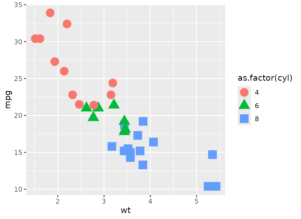
Now, let’s look at how we can use the color palette and theme with our base plot.
basePlot +

  # Use the color palette
  scale_color_dc() +

  # Get the ggplot theme
  theme_dc()
This plot now properly leverages the brand.
Other Options with color Aesthetic
Here are some other useful examples that demonstrate some of the function’s flexibility.
# Use the accent color palette instead of the fill
# This would be beneficial if you need to use the fill colors instead of the accent colors.
basePlot + scale_color_dc(overrideWithFill = TRUE) + theme_dc()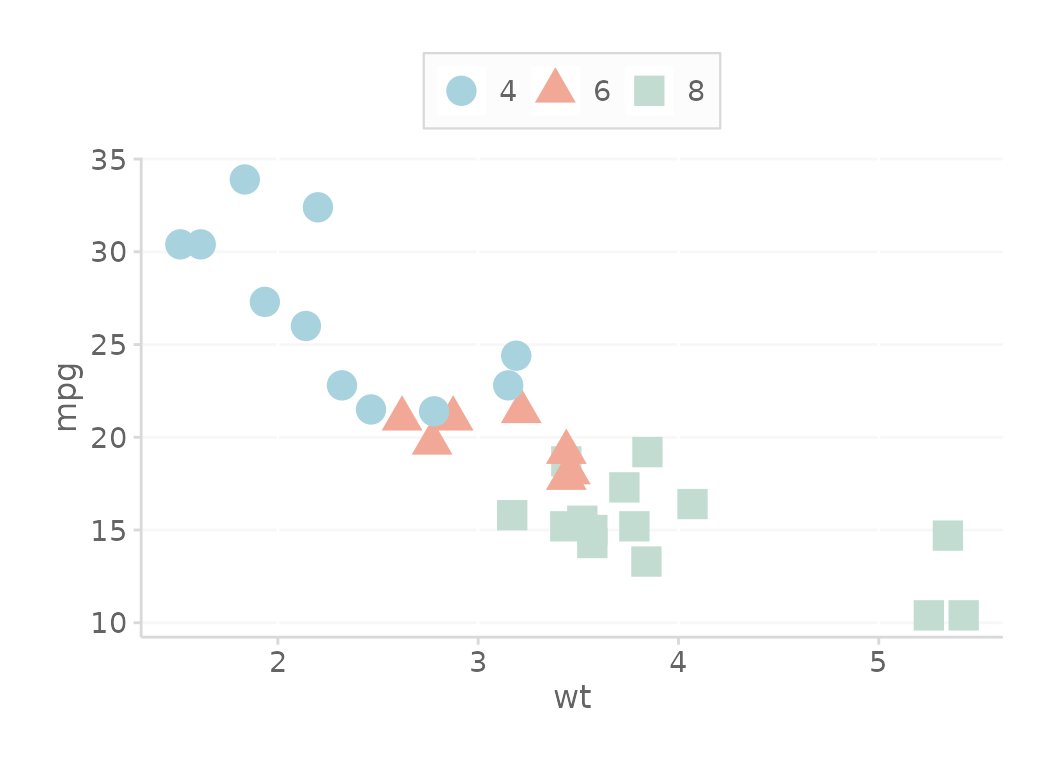
# Add the fill color and turn off legend with optional parameter
# You can use any parameter supplied through ggplot2::scale_fill_manual()
basePlot + scale_color_dc(guide = 'none') + theme_dc()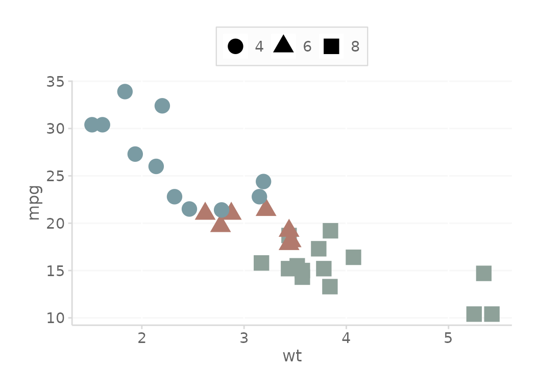
# You could also change the theme through the optional parameters
# Add the theme with additional optional theme parameters
basePlot + scale_color_dc() + theme_dc(legend.position = 'right')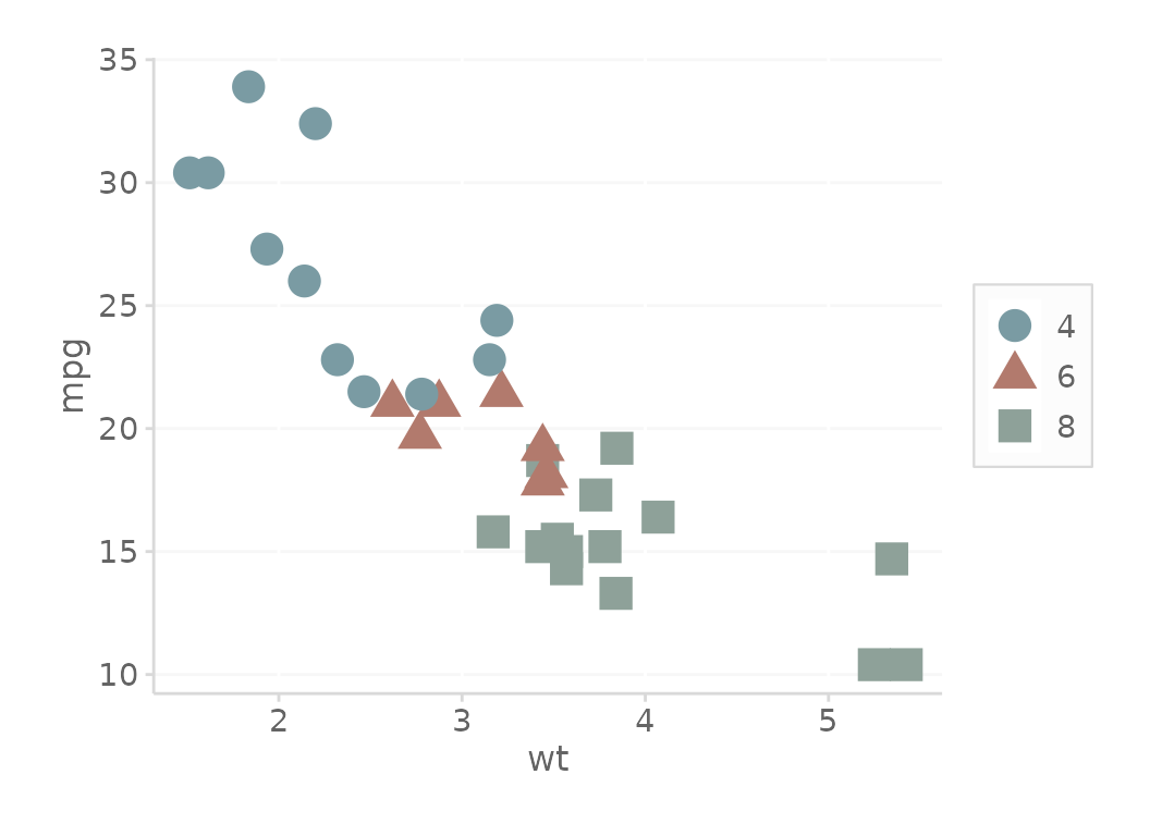
Additional parameter called borderMode controls the
theme borders. Inspiration
for facets came from 1.2.2 in this book.
# One other option is to remove the border when faceting
# Note this example is only for demonstrating the borders. Faceting in
# this context is another issue in itself.
basePlot + scale_color_dc() + theme_dc(borderMode = 'facet') +
  facet_grid(~as.factor(cyl))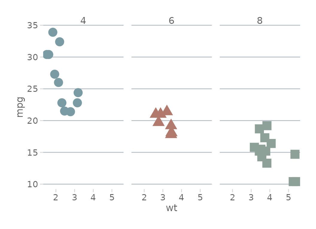
# Note you can also use 'borders' to add all border back.
basePlot + scale_color_dc() + theme_dc(borderMode = 'borders')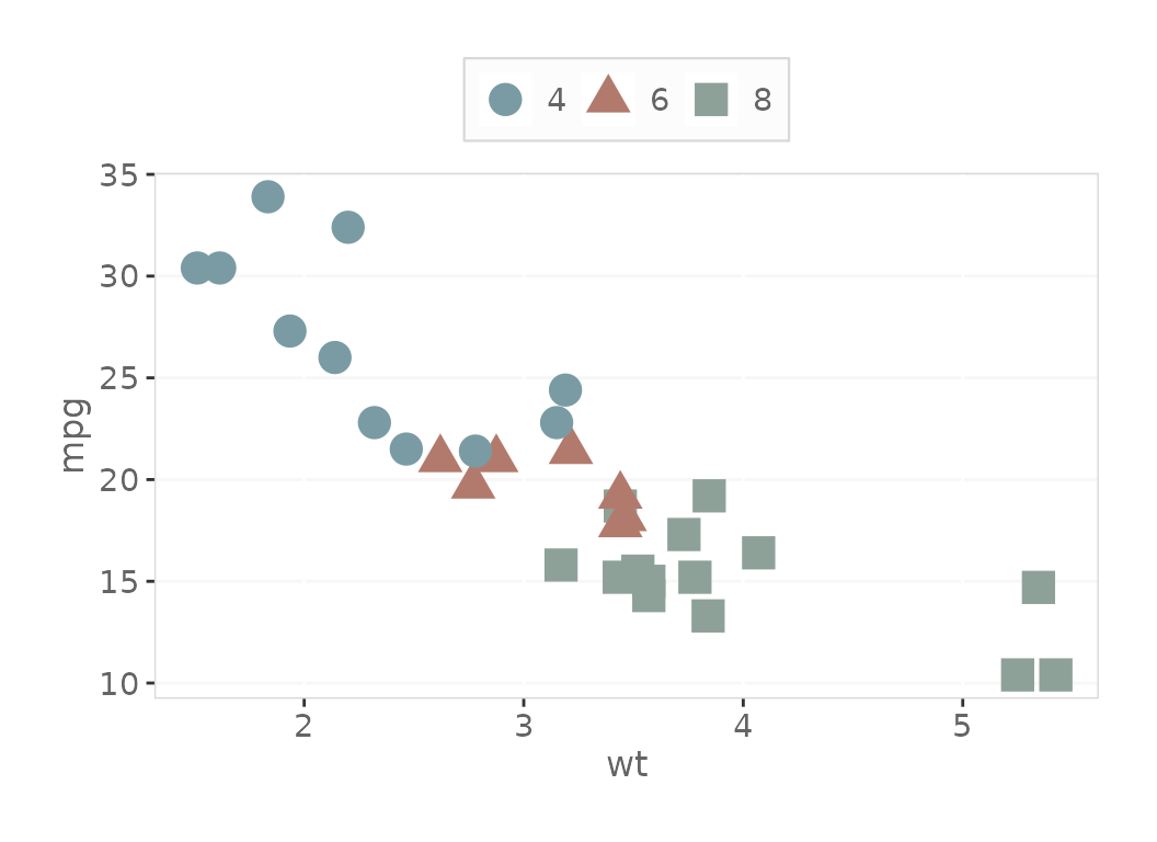
Use only 1 color
Most of the time you only need one color. Here is an example of how you might get that.
basePlot +

  # Use only a single color (note using line palette)
  geom_point(color = scale_dc('base', 'base2'),
             size  = 5) +

  # Get the ggplot theme
  theme_dc()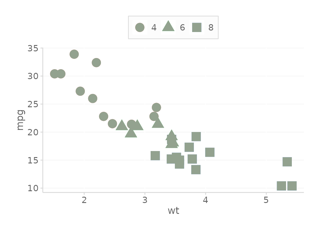
Adjusting fill Aesthetic
Here are some examples of how you could use the fill colors in plots.
Create a Base plot
# Create basic ggplot object
ggplotObject <- ggplot(mtcars, aes(y = mpg, x = as.factor(cyl),
                                   fill = as.factor(cyl), color = as.factor(cyl))) +

  # Note that gray border used for demonstration. Please use scale_color_dc()
  # as much as possible
  geom_boxplot(size = 0.8)
Here is the main combination that you might use.
# Add the fill and color
ggplotObject + scale_fill_dc() + scale_color_dc()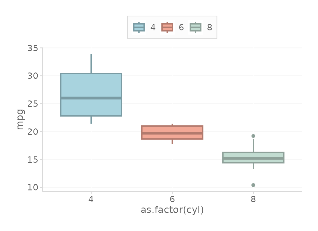
Below shows more options that demonstates some of the function’s flexibility.
# Create basic ggplot object
ggplotObject2 <- ggplot(mtcars, aes(y = mpg, x = as.factor(cyl), fill = as.factor(cyl))) +

  # Note that gray border used for demonstration. Please use scale_color_dc()
  # as much as possible
  geom_boxplot(size = 0.8, color = scale_dc('gray', 'gray3'))

# Add the accent color
ggplotObject2 + scale_fill_dc(overrideWithAccent = TRUE)
# Add the fill color and turn off legend with optional parameter
ggplotObject2 + scale_fill_dc(guide = 'none')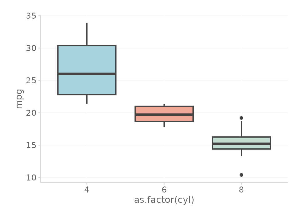
Darken Text when Over Filled Elements
ggplot(mtcars, aes(y = mpg, x = wt, color = as.factor(cyl))) +
  geom_point(aes(fill = as.factor(cyl)),
             size = 10,
             pch = 21,
             color = 'transparent',
             alpha = 0.9
  ) +
  geom_text(aes(label = round(mpg, 0))) +
  scale_fill_dc() +

  # KEY - darken the text so that it is easier to view
  # Over fill
  scale_color_dc(darkenPaletteForTextGeoms = TRUE) +
  theme_dc()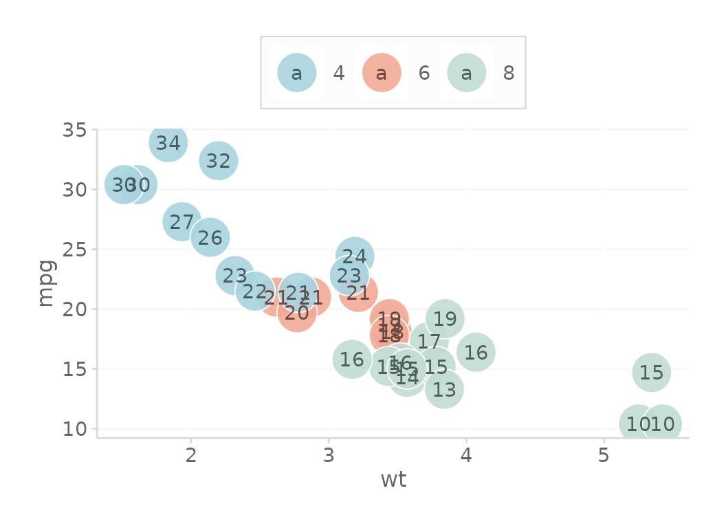
Offset or Reverse Order of Colors
# Offset the colors by 1
basePlot + scale_color_dc(colorOffset = 1)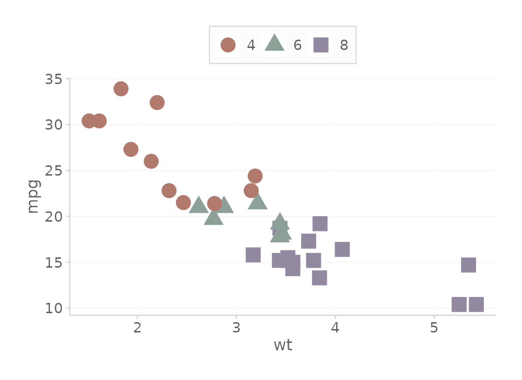
# reverse the order of the palette
basePlot + scale_color_dc(reverseOrder = TRUE)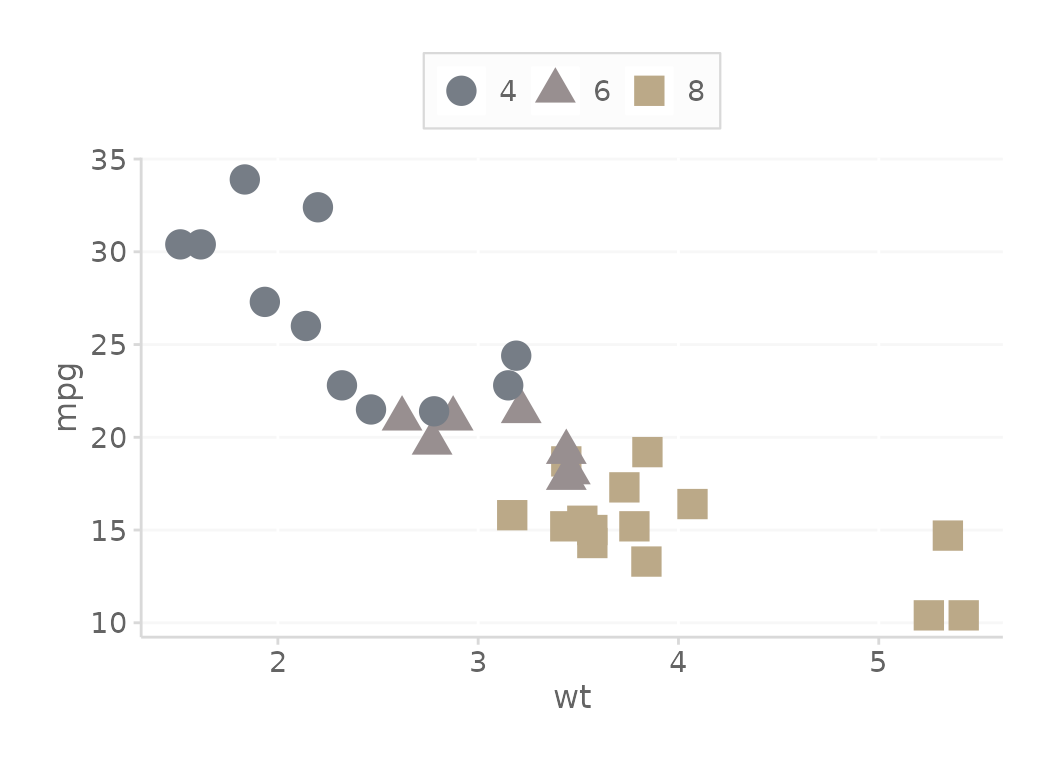
Override the palette with a color blind palette
# Use color blind friendly palette (works with fill too)
basePlot + scale_color_dc(useColorBlindPalette = TRUE)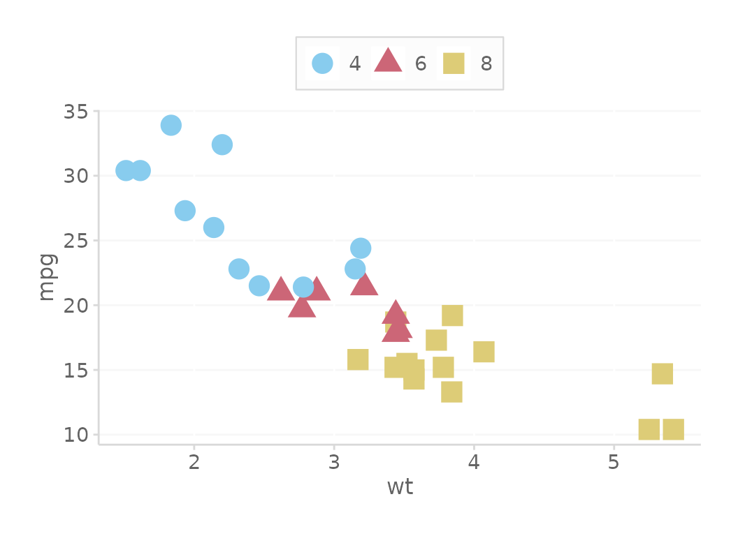
# Change the palette (can use cols4all::c4a_palettes() to try others)
# Also, can demo others in GUI using cols4all::c4a()
basePlot + scale_color_dc(useColorBlindPalette = TRUE,
                          colorBlindPaletteName = 'color_blind')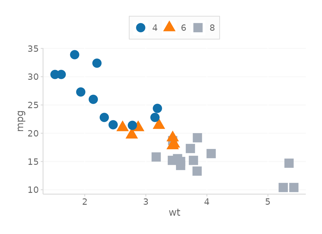
Numeric Formats
Mainly for quick financial axis formatting
kDollarsFormat(1000,          scaleUnit = 'K')
#> [1] "$1 K"
kDollarsFormat(1000000,       scaleUnit = 'M')
#> [1] "$1 MM"
kDollarsFormat(1000000,       scaleUnit = 'MM')
#> [1] "$1 MM"
kDollarsFormat(1000000000,    scaleUnit = 'B')
#> [1] "$1 B"
kDollarsFormat(1500000000000, scaleUnit = 'T')
#> [1] "$1.50 T"
kDollarsFormat(1000000,       scaleUnit = 'M', useDollarSign = FALSE)
#> [1] "1 MM"
Here are some examples of how you would commonly integrate them into
ggplot2
df <- mtcars
df$mpg <- df$mpg*1000000

# Create simple ggplot, no data shown by default
gg <- df |>
  ggplot(aes(y = mpg, x = wt)) +
  theme_dc()

# Text labels millions dollars
gg + geom_text(aes(label = kDollarsFormat(mpg)))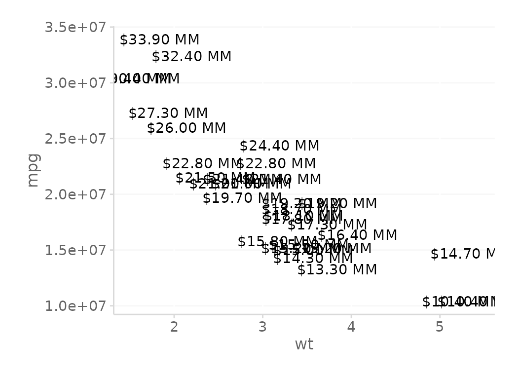
# y-axis format, using function defaults
gg + scale_y_continuous(labels = kDollarsFormat)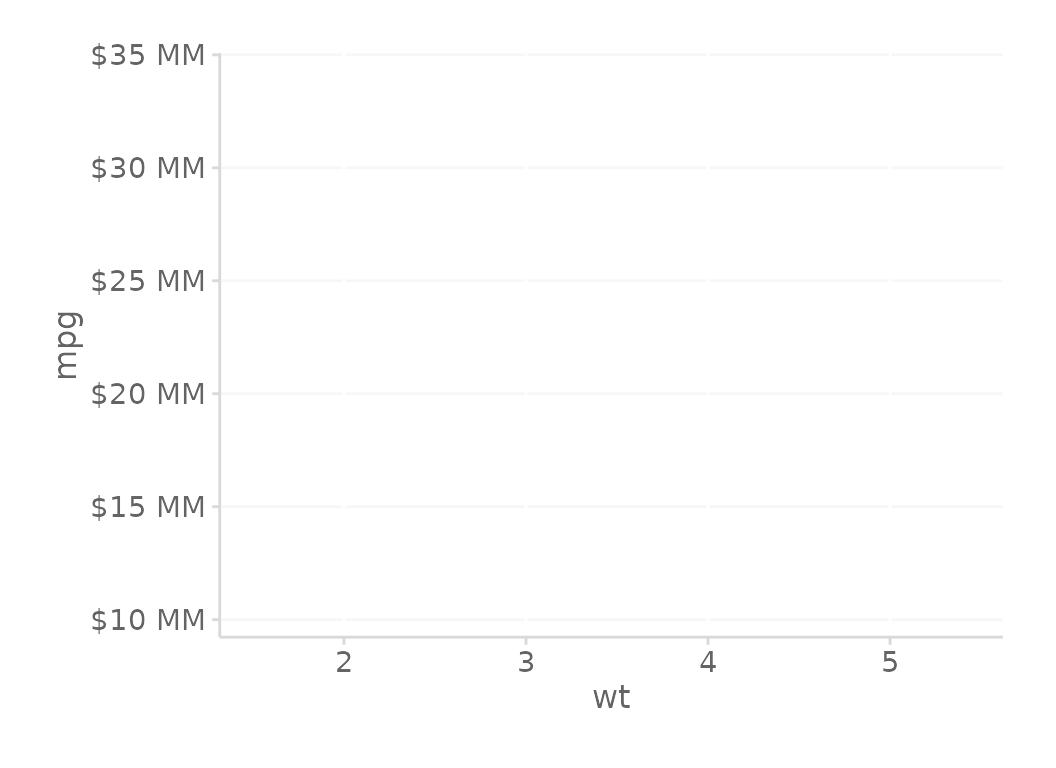
# y-axis format in *thousands* of dollars
gg + scale_y_continuous(labels = ~kDollarsFormat(., scaleUnit = 'K'))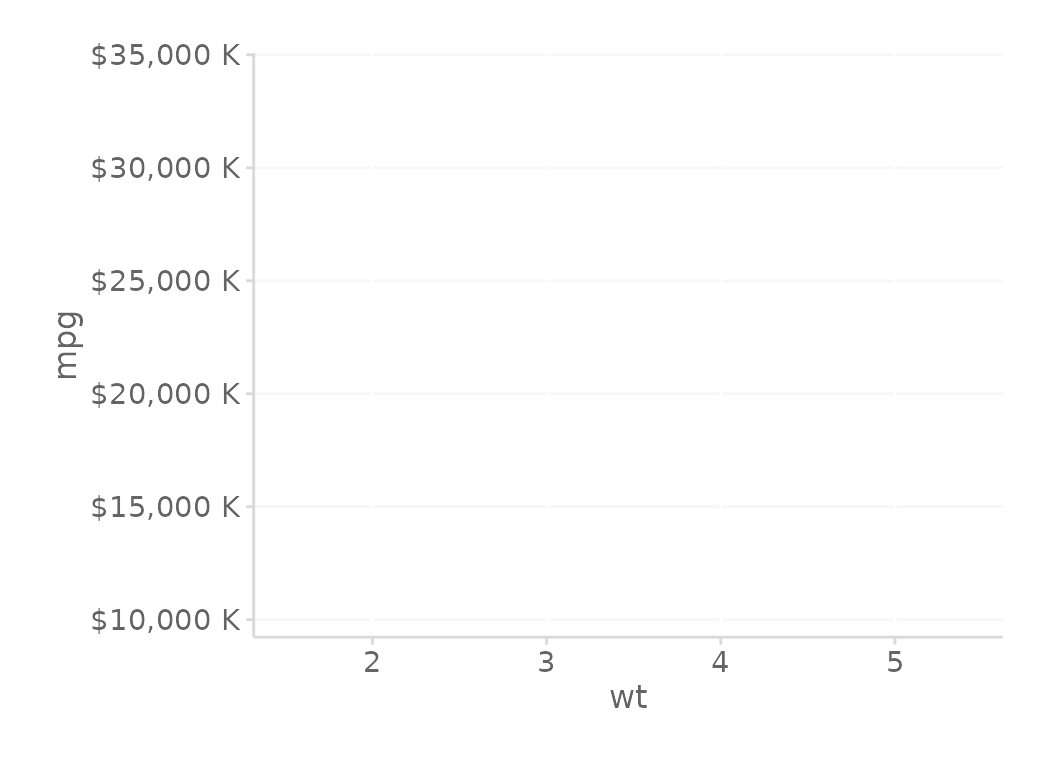
# y-axis format with no decimals
gg + scale_y_continuous(labels = ~kDollarsFormat(., roundToDigit = 0))
# y-axis format with no dollar sign
gg + scale_y_continuous(labels = ~kDollarsFormat(., useDollarSign = F))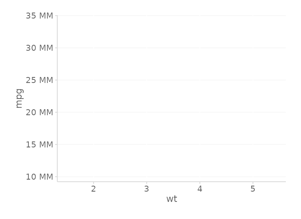
Colors Deep Dive
This section take a closer look at the colors that are available to
us in the styles package.
What Colors are Available?
Notice displayNames = TRUE, which show you what hex
codes are associated with the color names.
Default is displayNames = FALSE for best functionality
with plotting.
# Fill colors
scale_dc('fill', displayNames = TRUE)
#>      blue       red     green    purple    orange    yellow   purple1      gray
#> "#a8d3de" "#f2a896" "#c2dcd1" "#c7bbdb" "#f7d2b4" "#fee6ba" "#d0c3c5" "#a2acb7"

# Line colors
scale_dc('color', displayNames = TRUE)
#>      blue       red     green    purple    orange    yellow   purple1      gray
#> "#7a9ba3" "#b27a6d" "#8ea199" "#9289a1" "#b69a83" "#bba988" "#988f90" "#767d86"

# Blue and Gray colors, like the background of slide decks
scale_dc('base', displayNames = TRUE)
#>     base1     base2     base3     base4
#> "#bfd1ba" "#93a28f" "#596b59" "#3c493c"
scale_dc('gray', displayNames = TRUE)
#>     white    gray11    gray10     gray9     gray8     gray7     gray6     gray5
#> "#FFFFFF" "#FAFAFA" "#F5F5F5" "#F1F1F1" "#EAEAEA" "#D9D9D9" "#CFCECE" "#A6A6A6"
#>     gray4     gray3     gray2     gray1
#> "#646464" "#444444" "#363636" "#222222"

# Text, Grays, and Blues
scale_dc('text') # Text (dark gray)
#> [1] "#646464"
scale_dc('base') # Grays that are in the brand
#> [1] "#bfd1ba" "#93a28f" "#596b59" "#3c493c"
scale_dc('gray') # Blues that are in the brand
#>  [1] "#FFFFFF" "#FAFAFA" "#F5F5F5" "#F1F1F1" "#EAEAEA" "#D9D9D9" "#CFCECE"
#>  [8] "#A6A6A6" "#646464" "#444444" "#363636" "#222222"
How to get > 1 colors
# Get the first 3 colors in the line palette
scale_dc('color', 3)
#> [1] "#7a9ba3" "#b27a6d" "#8ea199"

# Get the last 3 colors in the fill palette
scale_dc('color')[6:8]
#> [1] "#bba988" "#988f90" "#767d86"

# Or access specific colors all at once
scale_dc('color', 'base', 'orange', 'green', 'yellow')
#> [1] "NA"      "#b69a83" "#8ea199" "#bba988"