Portfolio Optimization with Python Particle Swarm Optimizer

Particle Swarm Optimization is applied to portfolio choice modeling.

---

Note: Tickers are randomly selected

For demonstration only, the tickers are randomly chosen.

1 Presentation of Process and Research

---

2 Documentation of Process and Research

• Presentation Slides
• Research Paper
• Literature Review

---

3 Executed Code

3.1 Overview of Code

Class-based Python approach minimized portfolio risk and selected the max-Sharpe portfolio across simulations.

1. Inputs for model:

   • Stock tickers from publically traded companies, investment funds, etc. available on Yahoo Finance
     
   • Date range of Stocks to include in sample (Default last 10 years)
     
   • Minimum desired return on portfolio as a soft constraint
     
   • Some Metaheuristic inputs

2. StockFinanceMPT.py: Calls PullStockData.py to pull stock data, then prepares stock data to get excess returns, variance-covariance matrix, etc. for Modern Porfolio Theory. Must be in working directory

3. SimulateOptimalPortfolios.py:

   • Runs individual Particle Swarm Optimization routine, searching for the global minimum risk. Specifically, it creates many OptimizePortfolioPSO class objects.
     
   • Repeatedly simulate PSO modeling as desired.
     
   • Returns optimal allocation of weights to invest into stocks and associated investment weights.

4. ViewSimulatedPortfolios.py: Class that processes results of the simulations, which yields the following performance plots:

   • Displays variance characteristics across all simulations.
     
   • Across all simulations, plots:
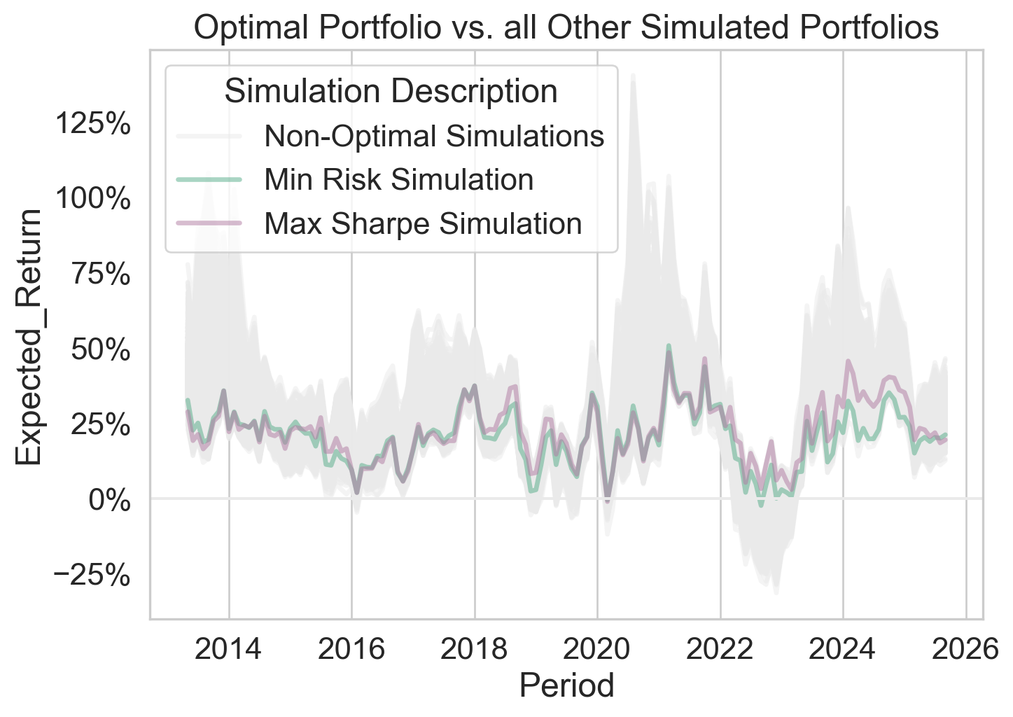
     • Global minimum risk portfolio and maximum Sharpe portfolios against all non-optimal portfolios.
       
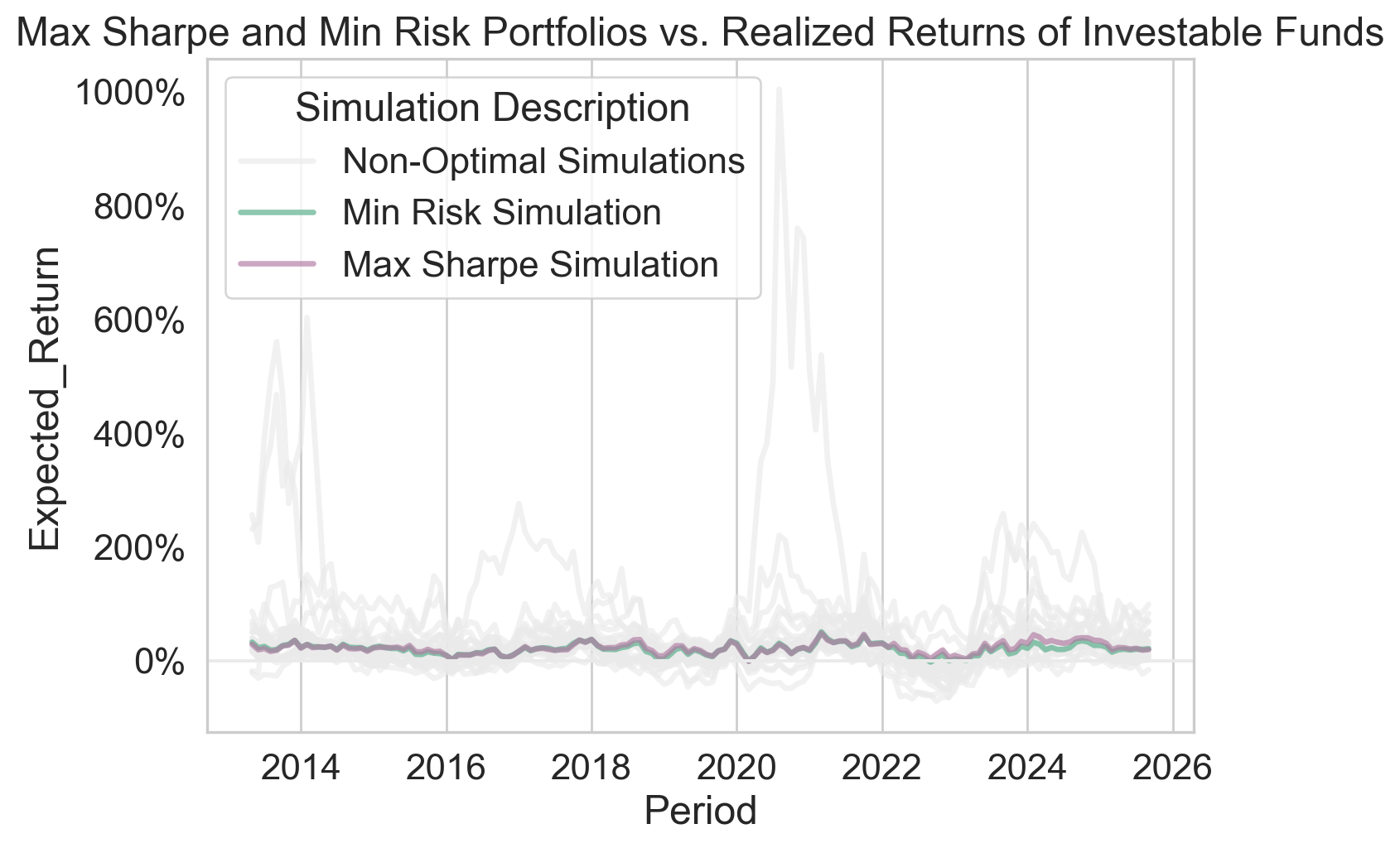
     • Global minimum risk portfolio and maximum Sharpe portfolios against all investable tickers, or funds.
       
   • Frontier of all simulated portfolios. I.e., risk vs. return of all simulated portfolios.

5. Exports CSVs of inputs, performance data, weights, etc.

---

# Set working directory to the R project directory
import sys
import os

sys.path.append(os.getcwd() + "//docs//02-Optimization//01-PSO-Portfolio//")

# Import custom classes
import datetime                  as dt  # For dates
import StockFinanceMPT           as mpt # Stock pull from yfinance in current wrkdir
import SimulateOptimalPortfolios as sop # Run simulations of global best portfolios
import ViewSimulatedPortfolios   as vsp # Wrapper class to plot, export, etc., simulations

3.2 Pull and Prepare Stock Data

Pulled price history and T-bill rates; built returns and covariance to power risk/return modeling.

See full function here.

# List of stock tickers to pull data
StockTickers = ['NVDA', 'MSFT', 'AAPL', 'AMZN', 'META', 
                'AVGO', 'GOOGL', 'GOOG', 'TSLA','JPM', 
                'WMT', 'V', 'LLY', 'ORCL', 'MA', 'NFLX', 
                'XOM', 'JNJ', 'COST', 'HD', 'BAC'
]

# Date range for stock & t-bill data pull - default last 10 years
maxDate = dt.datetime.today()                    # Max date to pull from
minDate = maxDate - dt.timedelta(days = 15*365) # Min date to pull from

# Pull stock data
PulledStockData = mpt.StockFinanceMPT(StockTickers, minDate, maxDate)

YF.download() has changed argument auto_adjust default to True

---

3.3 Run Particle Swarm Optimization

Simple Interpretation of Code: Start with 15 random portfolios, let each adjust 25 times while sharing results, and repeat 1,500 runs to identify both the minimum-risk and maximum-Sharpe portfolios.

See full function here.

# Create the simulation
simulatedPortfolios = sop.SimulateOptimalPortfolios(    
    PulledStockData,               # Using the pulled stock data above
    totalSimulations    = 1500,    # Number of min risk portfolio's to simulate
    totalIterations     = 25,      # Total number of iterations (or movements within one simulation)
    numPorfolios        = 15,      # Total number of portfolios in a swarm. 
    minDesiredReturn    = 0.07     # Targeted expected return, soft constraint
    )

simulatedPortfolios.runSimulation() # Run the simulation given parameters above

---

4 View Results

4.1 Review Minimum Risk Portfolio

Identified the minimum-risk mix as the baseline; quantified risk reduction versus the starting set.

See full function here.

# Create the viewer wrapper class
simulationViewer = vsp.ViewSimulatedPortfolios(simulatedPortfolios, displayResults = False)

---

4.2 Compare Optimal Portfolio to the Efficient Frontier

Placed the chosen portfolio on the frontier to confirm its risk/return position.

See full function here.

simulationViewer.plotRiskVsReturnVsSharpe(TRANSPARENCY_LEVEL=0.33)

---

4.3 Compare Optimal Portfolio to All Other Simulated Portfolios

Benchmarked the optimal result against all simulations to validate consistency and uplift.

See full function here.

simulationViewer.plotOptimalVsNonOptSimulations()

Note that the min risk portfolio is the same as the sharpe portfolio!

---

4.4 Compare Optimal Portfolio to All Investable Assets

Showed diversification benefits versus single assets; improved return per unit of risk.

See full function here.

simulationViewer.plotOptimalVsRealizedReturns()

Note that the min risk portfolio is the same as the sharpe portfolio!

---

4.5 Other Class Functions

Exported data and plots; enabled quick checks and repeatable reporting.

See full function here.

# Exports all Weights Data and Plots to dated folder
simulationViewer.exportSimulationData()

Input_Parameters saved to:       Output_Data/2025-09-07 09_50/Input_Parameters.csv
All_Simulated_Weights saved to:      Output_Data/2025-09-07 09_50/All_Simulated_Weights.csv
All_Simulated_Weights_Stats saved to:        Output_Data/2025-09-07 09_50/All_Simulated_Weights_Stats.csv
Min_Risk_Portfolio saved to:         Output_Data/2025-09-07 09_50/Min_Risk_Portfolio.csv
Max_Sharpe_Portfolio saved to:       Output_Data/2025-09-07 09_50/Max_Sharpe_Portfolio.csv
Expected_Returns saved to:       Output_Data/2025-09-07 09_50/Expected_Returns.csv
Expected_Returns_Stats saved to:         Output_Data/2025-09-07 09_50/Expected_Returns_Stats.csv

See full function here.

# Inspect that the sum of weights constraint is met (100%)
simulationViewer.checkSumOfWeights()

# Invested Variability among assets
simulationViewer.plotPortfolioVarianceStats(figHeight=7, figWidth=5)

# Process all output at once
simulationViewer.processAllOutputAtOnce()